Factored Representations, in Fruit
July 7, 2026
Note to self. This week I went after F2 — a stress-test of the "factored representations" story from Shai et al. I like this paper a lot, which is exactly why it's fun to try to break. And I thought I had: I pushed it to high factor count and watched the clean picture fall apart. Then I found out the picture wasn't falling apart at all — I was just measuring it wrong, in a way that took me a while to see. So this is half a paper walkthrough and half a confession. Let me start with the fruit, because it's the only way I know how to keep the whole thing straight in my head.
Five fruit vendors
Picture a street corner with five fruit vendors standing in a row. Each vendor has their own private mood that drifts around over the day, and once every second, all five of them shout a fruit at the same time. What you hear isn't five clean shouts — it's one blurted-together composite. You write down which composite you heard as a single number, and that number is your whole dataset. A stream of integers. That's all the model gets too.
If a model tracks a bunch of independent "factors" and each one lives in its own orthogonal subspace, then a steering vector is (roughly) editing one thing. If they don't, every activation-patching result that assumes "I'm editing one thing" is quietly editing several at once. So "do the subspaces stay orthogonal as you add factors" is load-bearing for a lot of interp tooling — it's the reason I bothered pushing on this.
Each vendor is a little state machine — formally a generalized hidden Markov model, a tuple $\mathcal{M}_n = (\mathcal{X}_n, \mathcal{S}_n, \boldsymbol{\eta}^{(\varnothing)}_n, (T_n^{(x)})_x)$: the fruits it can shout $\mathcal{X}_n$, its space of moods $\mathcal{S}_n$, where it starts, and a set of matrices $T_n^{(x)}$ that say how its mood updates when it shouts fruit $x$. Don't worry about the tuple; the vendor is the intuition.
Anatomy of one vendor
Three of the five vendors are what the paper calls mess3 factors. Each one has exactly three pieces.
Three moods. Call them 🍎-mood, 🍌-mood, 🍐-mood. At any instant the vendor is in exactly one, and you can't see which — that's the "hidden" in hidden Markov. Only the vendor knows.
An emission rule. When it's time to shout, the vendor picks a fruit from a distribution that depends on its current mood — and crucially, not deterministically:
- 🍎-mood → 80% 🍎, 10% 🍌, 10% 🍐
- 🍌-mood → 10% 🍎, 80% 🍌, 10% 🍐
- 🍐-mood → 10% 🍎, 10% 🍌, 80% 🍐
So 🍎-mood "mostly means apple, but sometimes lies." That little bit of lying is the whole reason the problem is interesting — two apples can come out of different moods, and telling them apart is the inference the model has to do.
A transition rule. After shouting, the vendor moves to a new mood — again from a mood-dependent distribution, and mostly it just stays put:
- from 🍎-mood → 80% stay 🍎, 10% drift 🍌, 10% drift 🍐
- from 🍌-mood → 10% 🍎, 80% stay 🍌, 10% 🍐
- from 🍐-mood → 10% 🍎, 10% 🍌, 80% stay 🍐
That's the entire vendor. Three moods, an emission rule per mood, a transition rule per mood, all of it invisible to you. A run looks like long stretches of one fruit with the occasional "wrong" shout mixed in:
mood: 🍎 🍎 🍎 🍎 🍌 🍌 🍌 🍐 🍐 🍐 🍎 🍎
shout: 🍎 🍎 🍎 🍌 🍌 🍌 🍐 🍐 🍐 🍎 🍎 🍎
The other two vendors are tom_quantum factors — Shai calls them "Bloch Walk." Same idea, just three moods mapped onto a four-fruit menu (🍇, 🥭, 🍋, 🥝) with messier emission numbers. Different shape, same story: hidden mood, probabilistic shout, drifting transitions.
The composite you actually hear
Now stack all five. Every second the corner emits a tuple — one fruit per vendor — and the joint machine's transition operator is just the tensor product of the individual ones:
$$T^{(x)} = \bigotimes_{n=1}^{5} T_n^{(x_n)}$$There are $3 \times 3 \times 3 \times 4 \times 4 = 432$ possible tuples. The street has a sign that assigns each tuple an arbitrary integer from 0 to 431 — no relationship between neighbouring integers, the mapping is scrambled on purpose. That integer (plus a start-of-sequence marker, so vocab size 433) is what lands in your notebook. Then I train a vanilla 4-layer GPT-2-style transformer on the stream with plain next-token cross-entropy. Nothing tells it there are five vendors, what fruit is, or that composite #47 unpacks to (🍎, 🍌, 🍎, 🥭, 🥝). It sees integers.
What the model has to compute
To predict the next composite well, the ideal predictor has to reconstruct, after every history, each vendor's current belief over its own moods — a point on a little triangle (a 2-simplex). Bundle all five together and you get the system's predictive vector:
$$\boldsymbol{\eta}^{(x_{1:\ell})} = \frac{\boldsymbol{\eta}^{(\varnothing)} T^{(x_1)} \cdots T^{(x_\ell)}}{\boldsymbol{\eta}^{(\varnothing)} T^{(x_1)} \cdots T^{(x_\ell)} \mathbf{1}}$$which naïvely lives in the joint space of dimension $\prod_n d_n = 3^5 = 243$ (242 after you account for it being normalized). That's the "dumb" way to hold it — one coordinate per joint mood.
$242 \to 10$. Because the vendors are independent, the joint belief is always the product of the five little triangles — so you never need the full 243-way table, just five 2-dimensional points. Exponentially smaller, and (when the factors really are independent) exactly lossless.
But the vendors are independent, so the belief always factors — it's a product state, $\boldsymbol{\eta} = \bigotimes_n \boldsymbol{\eta}_n$ — which means all the information is already sitting in the five individual triangles $\boldsymbol{\eta}_n$. Line them up side by side instead of multiplying them out,
$$\boldsymbol{\eta}_{\text{FWH}}^{(x_{1:\ell})} \equiv \bigoplus_{n=1}^{5} \boldsymbol{\eta}_n^{(x_{1:\ell})}$$and now you're in $\sum_n (d_n - 1) = 5 \times 2 = \mathbf{10}$ dimensions. Two per vendor, five vendors, ten total. 242 → 10. Exponential compression, and lossless whenever the factors are conditionally independent.
The claim (the Factored World Hypothesis)
Here's the bet. A transformer with $d_{\text{model}} = 120$ has tons of room for the fat 242-dim joint belief. There's no capacity reason to prefer the skinny 10-dim factored one. The FWH says it goes factored anyway — and more than that, it puts each vendor's triangle in its own roughly-orthogonal 2-dim slab of the residual stream. Five slabs $V_1, \dots, V_5 \subset \mathbb{R}^{120}$, with $V_n \perp V_m$, each carrying one vendor's belief and none of the others'.
Two things "orthogonal" does not mean, because I tripped on both. It's not "every concept is orthogonal to every other concept" — that's geometrically impossible in a real LM tracking millions of things. It's orthogonality between the subspaces of whole independent generative processes (a handful of them: think tense, register, speaker identity), which is at least feasible in a wide residual stream. And even at $N=5$ it's approximate — Shai's own cleanest figure has ~2 dims of overlap.
The deeper claim — an inductive bias, not just efficiency (with the Bayes bit)
The part that makes FWH more than "compression is nice" is Section 4.3: the model doesn't just land on the factored solution, it routes through it first, even when factoring is a bad idea. The test is a noisy channel — with probability $\varepsilon$ the composite you observe is replaced by a uniform-random integer, so $T^{(x)} = \varepsilon T_{\text{int}} + (1-\varepsilon)\bigotimes_n T_n^{(x)}$. Now factoring is genuinely lossy.
Why lossy, when the vendors are still independent? Because the shared noise flag couples them in the posterior. Tiny worked example: two vendors, moods A/B, each emits its "home" fruit 90% of the time, both 95% likely to be in A. You observe (🍌, 🍌) under $\varepsilon = 0.2$. Grinding the Bayes over {AA, AB, BA, BB} × {faithful, noise} and marginalizing out the noise flag gives $P(V_1=A)=0.783$, and $P(BB) = 0.027$ — but a factored belief could only ever produce $P(BB) = P(B)^2 = 0.115^2 = 0.013$. The joint puts extra mass on the "both flipped together" corner, because either the whole composite was corrupted or none of it was. That shared flag ties the vendors together via explaining-away even though their dynamics never touch.
(If the noise were per-vendor instead of per-composite, the coupling vanishes and factored beliefs stay exactly right — so it's specifically the composite-level corruption that makes this bite.)
And the finding: no matter what $\varepsilon$ is, the residual stream's effective dimension collapses to ~10 within a few hundred steps and dwells there before (at high $\varepsilon$) expanding later. It visits factored first, every time. Shai calls it an attractor. That's the real claim, and it's the thing I'd most want to push on next — crank $\varepsilon$ to $0.8$ where factored is badly wrong, and see if the model still can't help itself.
Reproducing it
Before attacking anything, does the basic picture even come out on my own models? I cloned the paper's reference repo for the data and trained the canonical 4-layer transformer ($d_{\text{model}}=120$, joint softmax over the composite vocab) on the 2–8 factor regimes.
First check is cumulative explained variance: how many principal directions of the residual stream you need to capture 95% / 99% of its variance. FWH predicts $\approx\sum_n d_n$, not $\prod_n S_n$. It lands — 2 factors need ~5 directions, 4 need ~10, and it doesn't budge even when I widen the model to $d_{\text{model}}=480$ and hand it twenty times the room it needs.
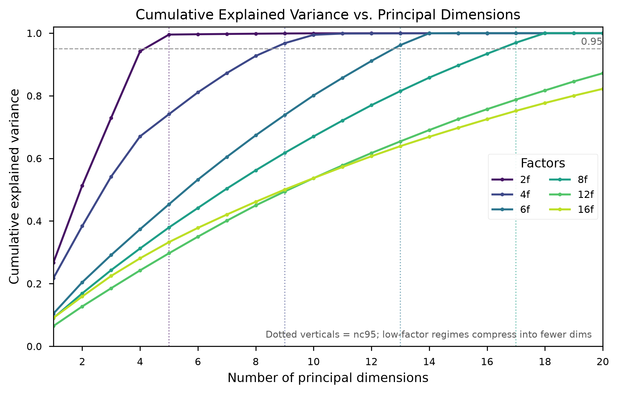 CEV per regime. Variance concentrates in $\sum_n d_n$ dimensions — the compression claim, reproduced.
And the prettiest one — belief geometry. Train a 5-factor model, and for each vendor plot its true belief triangle next to the belief you can linearly recover from the residual stream.
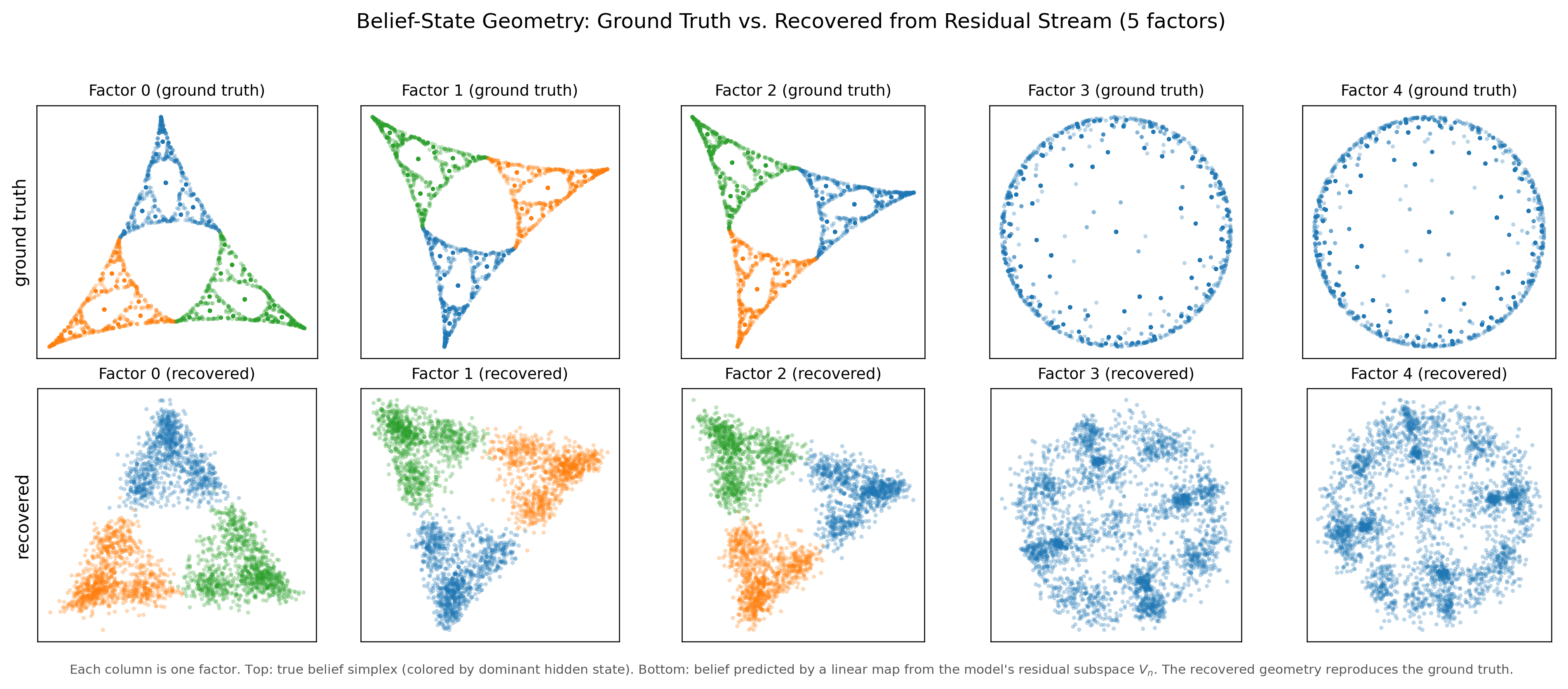 Top: the ground-truth belief triangle per vendor — the three
 mess3 factors trace that Sierpinski fractal, the two Bloch-Walk ones fill a disk. Bottom: the belief recovered by a linear read-out, decode $R^2 = 0.99$ on every factor. The residual stream carries the full geometry, linearly. Everything downstream rests on this landing cleanly — which, spoiler, is exactly where I got into trouble.
The thing I thought I'd found
Reproduction's fine. So I did the part the paper doesn't — pushed $N$ up, to $\{2, 4, 6, 8, 12, 16\}$, and asked whether the orthogonality survives. My first pass said: no, it degrades. Pairwise subspace overlap climbing to $0.8$ by 16 factors, and a "forced orthogonalization" test — Gram-Schmidt the subspaces apart, measure how much decode $R^2$ you lose — stripping ~48% of the signal at 16f. Looked like a real large-$N$ breakdown. I was ready to write it up as "factored representations don't scale."
It wasn't a breakdown. It was me measuring the subspaces wrong, and the way I was wrong is genuinely the interesting part, so let me actually explain it instead of just fixing the number.
Where I fooled myself: decode vs. encode
There are two ways to pull "vendor $n$'s subspace" out of the residual stream, and I'd quietly assumed they were the same thing:
- Decode (regression). Regress the known belief$_n$ onto the activations and take the coefficient directions. These are the directions a linear reader leans on to recover the factor.
- Encode (vary-one). Hold the other four vendors fixed, sweep vendor $n$, and take the directions the activations actually move along. These are where the model writes the factor. This is the paper's method — and I'd skipped it for the easier regression.
You'd expect these to basically coincide. On these models they're almost orthogonal to each other — principal cosines around $0.001$ — even though both decode the belief at $R^2 \approx 1$. How is that possible? The residual stream here is wildly anisotropic and low-rank — something like 17 active dimensions out of 256. Least-squares is perfectly happy to read a factor out of a tiny-variance direction that just happens to correlate with it, while the model is writing that factor into a big, load-bearing direction. Both "work" as decoders. They point completely different ways. And the overlap you compute depends entirely on which one you decided to call "the subspace."
A random 2D slice of the residual stream still decodes belief$_n$ at $R^2 \approx 0.02$ — so the factor really is in a genuine low-dim subspace, it's not smeared everywhere. It's just that there are (at least) two different low-dim subspaces that both decode it, and they're nearly perpendicular. The regression one is a decoder's convenience. The vary-one one is where the representation actually lives. FWH is a claim about the representation.
So the forced-orthogonalization number gives you completely different answers depending on the basis. Same models, both estimators, using the paper's real overlap metric ($\sum_i\sigma_i^2/\min\dim$ — the mean squared principal cosine, an honest $[0,1]$ alignment measure, not the max-cosine I'd reported before):
| model | decode overlap | decode E1 $\Delta R^2$ | encode overlap | encode E1 $\Delta R^2$ |
|---|---|---|---|---|
| 2f (joint, d=120) | 0.02 | −0.02 | 0.005 | +0.00 |
| 4f (joint, d=120) | 0.05 | −0.23 | 0.010 | +0.02 |
| 6f (factored, d=256) | 0.10 | −0.26 | 0.009 | +0.02 |
| 8f (factored, d=256) | 0.05 | −0.26 | 0.010 | +0.04 |
| 8f (factored, d=64) | 0.11 | −0.49 | 0.022 | +0.10 |
| 12f (factored, d=256) | 0.06 | −0.42 | 0.023 | +0.04 |
| 16f (factored, d=256) | 0.72 | −0.64 | 0.045 | +0.08 |
The decode columns reproduce my scary trend — overlap and $|\Delta R^2|$ both climb with $N$, and at 16f you "lose" nearly two-thirds of the signal. The encode columns are flat and near-zero at every factor count, 16f included ($+0.08$, same band as everything else). In the subspace the model actually writes each factor into, the factors stay orthogonal, and forcing them orthogonal costs nothing. The whole large-$N$ degradation lived in the regression readout. It was never a fact about the model.
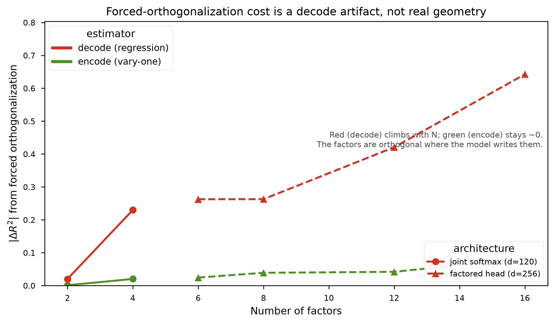 The whole correction on one plot. Red = decode (regression) E1, green = encode (vary-one) E1; the two line styles are the two architectures (see below), never merged into one curve. Red slides down with $N$; green sits at $\approx 0$. The factors are orthogonal where the model writes them.
A second test, "E4," backs this up: project one vendor's whole subspace out and see how much it damages the other vendors' decode. It's clean — strongly diagonal, off-diagonal mean $\le 0.02$ even at 16f. Ablating one factor barely touches the rest, and with the causal E1 also $\approx 0$, the two agree instead of fighting. (They did fight under the decode basis, which in hindsight was the tell — two of your metrics disagreeing usually means one is measuring an artifact.)
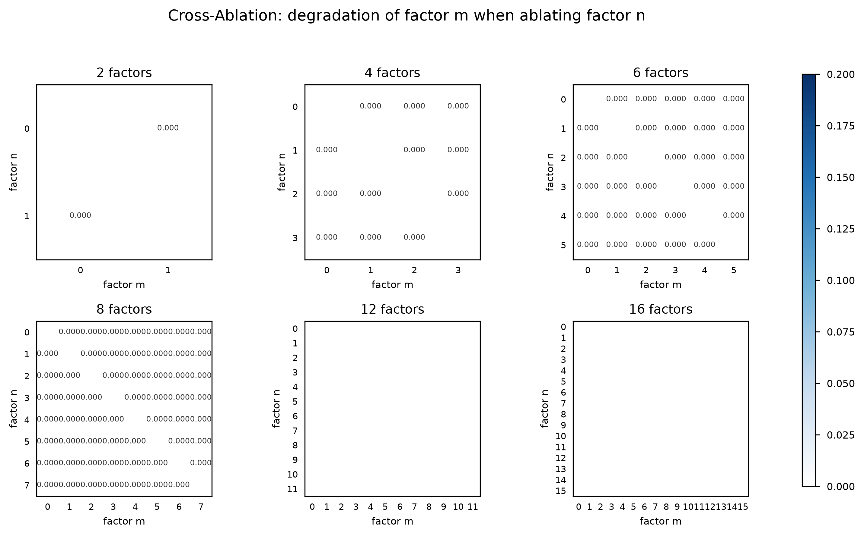 E4 cross-ablation. Bright diagonal, dark everywhere else, at every regime — ablating vendor $n$ mostly hurts vendor $n$.
A confound, and a bonus
One more thing was wrong with the original scan, and chasing it turned up something I didn't expect. The 2–8f models use a joint softmax over the composite vocabulary; at 12f/16f that vocabulary explodes (76 million tokens at 16f — the unembedding alone would be a 40-billion-parameter matrix), so those regimes had quietly switched to a factored head — one small softmax per vendor. Plotting all six points on one line pretends $N$ is the only thing changing. So now I draw them as two labelled lines that share $N=8$ as an anchor.
And the surprise: the joint-softmax 8f model isn't just slow, it's optimization-limited. An 11,664-way softmax with 8 factors gives each class about $0.02$ supervised examples per batch — a genuinely nasty landscape. It plateaus at loss $\approx 9.4$ (optimal is ~7) and only decodes at $R^2 \approx 0.25$ even after 60k steps, a wider model, and LR warmup. So the joint picture doesn't just become memory-intractable past ~10 factors — it becomes optimization-hard already at 8, which is a small argument in its own right for why a real system juggling many attributes would reach for factored readouts.
The width sweep, reinterpreted
I also swept $d_{\text{model}}$ at $N=8$ to ask "is the orthogonality just spare-dimension slack?" The decode E1 does slide with width — $-0.49$ at $d{=}64$ up to $-0.19$ at $d{=}512$ — but the encode E1 is flat and $\approx 0$ at every width. Same story as the $N$ sweep: the width dependence is a property of the least-squares decoder, not the representation. The model writes the factors orthogonally regardless of width; only the decoder's reliance on shared low-variance junk changes.
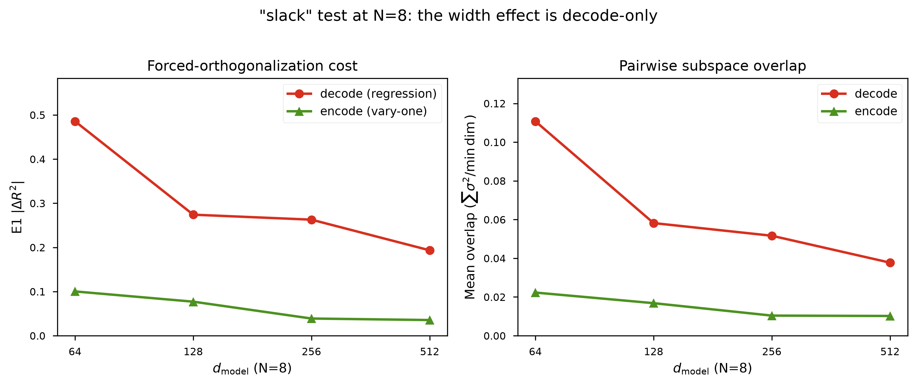 $d_{\text{model}}$ sweep at $N=8$. Decode (red) slides with width; encode (green) flat at ~0. The width dependence is decode-only.
Does a real model do this?
The toy is clean, but I wanted to see the phenomenon somewhere real. The right question isn't about correlated attributes — a bleed test between correlated things is rigged, correlation forces shared geometry by construction. It's whether structurally independent axes land in orthogonal subspaces. So: four genuinely independent grammatical dimensions of English, each with a minimal-pair contrast set that varies just that axis —
- number — "The dog runs" vs. "The dogs run"
- tense — "She walks" vs. "She walked"
- negation — "She walked" vs. "She didn't walk"
- voice — "The cat chased the mouse" vs. "The mouse was chased by the cat"
Each axis's direction is the diff-of-means of GPT-2-small's residual stream (layer 9, last token), normalized. All four decode cleanly (ridge $R^2$ 0.88–0.96), and the thing I actually care about is the $4\times4$ matrix of $|\cos\angle|$ between them.
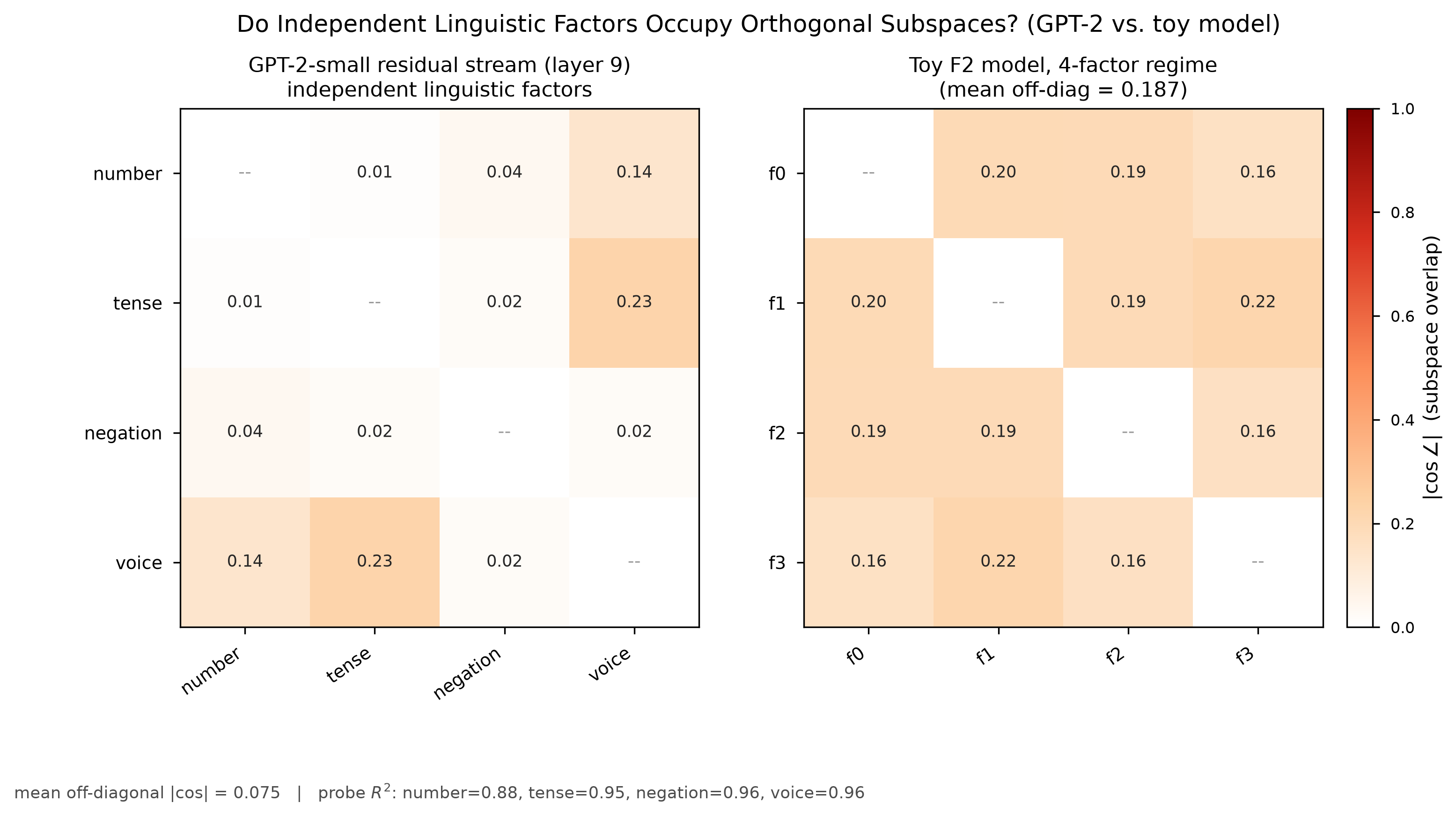 Off-diagonal $|\cos\angle|$ between the probe directions. Left: GPT-2-small, layer 9 — mean off-diagonal $|\cos| = 0.075$, max $0.23$. Right: the toy F2 model, 4-factor regime, same scale. Four independent grammatical factors sit in near-orthogonal subspaces in a model nobody trained on hand-built factors.
I read these off the last token, not a mean over tokens: mean-pooling bleeds a shared "sentence got longer" signal into negation and voice and spikes their overlap to $0.93$ (last-token: $0.02$). Same trap as decode-vs-encode — a readout choice masquerading as geometry.
What I actually learned
The headline I started with — "factored representations don't scale" — was just wrong, and wrong in a way worth keeping. Every piece of the "degradation" was a measurement artifact: a max-cosine number dressed up as alignment, and a regression decoder standing in for the representation on a residual stream low-rank enough that the two come apart hard. Measured the paper's own way — vary-one, and the real overlap metric — the factored, orthogonal-subspace picture is robust from 2 to 16 factors. The sharp prediction holds further than I gave it credit for.
But the useful takeaway is the caution, not the scare. On a low-rank residual stream, "the subspace for attribute $X$" is estimator-dependent — a regression probe and a causal vary-one probe can hand you two near-orthogonal subspaces that both decode perfectly. If you build a steering vector on the regression-probe subspace, you can eat collateral effects (that decode-side E1) that aren't in the representation at all. So the practical warning for steering and patching does survive — it's just a warning about your probe, not about the model's geometry. Identify the subspace causally, and the collateral goes away.
tl;dr
Compression + low-$N$ orthogonality: reproduce. My "orthogonality degrades at high $N$" claim: retracted — it was a max-cosine framing plus a regression-decoder artifact on a low-rank residual stream. Measured causally (vary-one), forced-orthogonalization costs $\approx 0$ at every factor count and width; E1 and E4 agree; the factored picture holds to 16 factors. GPT-2 keeps four independent grammatical factors near-orthogonal (mean off-diag $|\cos| = 0.075$). Real lesson: "the subspace for X" is estimator-dependent — identify it causally before you edit it.
— F2, wrapped. Onto the VLAs.